imshow#
This section describes various options available for imshow plots in fivecentplots
Setup#
Import packages:
[ ]:
import fivecentplots as fcp
import pandas as pd
from pathlib import Path
import imageio.v3 as imageio
import itertools
Load a completely ridiculous 8-bit RGB color test image as a np.array:
[ ]:
img_rgb = imageio.imread(str(Path(fcp.__file__).parent / 'test_data/imshow_cat_pirate.png'))
img_rgb
array([[[223, 221, 220],
        [223, 221, 220],
        [223, 221, 220],
        ...,
        [222, 220, 219],
        [222, 220, 219],
        [222, 220, 219]],

       [[223, 221, 220],
        [223, 221, 220],
        [223, 221, 220],
        ...,
        [222, 220, 219],
        [222, 220, 219],
        [222, 220, 219]],

       [[223, 221, 220],
        [223, 221, 220],
        [223, 221, 220],
        ...,
        [222, 220, 219],
        [222, 220, 219],
        [222, 220, 219]],

       ...,

       [[ 86,  95, 108],
        [ 84,  93, 106],
        [ 81,  90, 103],
        ...,
        [210, 211, 209],
        [210, 211, 209],
        [210, 211, 209]],

       [[ 85,  94, 107],
        [ 83,  92, 105],
        [ 81,  90, 103],
        ...,
        [211, 212, 210],
        [211, 212, 210],
        [211, 212, 210]],

       [[ 84,  93, 106],
        [ 83,  92, 105],
        [ 81,  90, 103],
        ...,
        [211, 212, 210],
        [211, 212, 210],
        [211, 212, 210]]], dtype=uint8)
Input data format#
fivecentplots was originally designed to simplify plotting from 2D pandas.DataFrames. However, this approach is not convenient or efficient for storing / displaying / processing image data, especially for color images with 3 or more channels of pixel data. Starting with v0.6.0, fivecentplots adopts a new convention that is significantly faster, particularly when grouping across multiple images:
Single images without any grouping labels:
Image data is passed to the plotting function through the its first and only required arg
Option 1 (recommended): image data is stored in
numpyarray → works with 2D grayscale/RAW image and RGBA color images (3 or 4 channels)img = imageio.imread('some_image_file.png') # np.array fcp.imshow(img, **kwargs)Option 2: image data is stored in a 2D
pd.DataFramewith integer labeled columns and integer labeled row indices → works for 2D grayscale/RAW onlyimg = pd.DataFrame(imageio.imread('some_image_file.png')) # pd.DataFrame fcp.imshow(img, **kwargs)
Grouping label information:
stored in a
pd.DataFrameeach grouping label is a column in the
pd.DataFrameone row for each image
row index is a unique key / name / number that corresponds to the image data
Image data:
stored as a dictionary of
np.arrayseach dictionary key matches a row index value for the grouping
pd.DataFramedictionary is passed to special kwarg named
imgs
Examples of both cases are provided below.
df = pd.DataFrame({'alpha_blend': [1, 10, 50], 'gamma': [1, 2.2, 1.8]}, index=['img0', 'img1', 'img2'])
df
| alpha_blend | gamma | |
|---|---|---|
| img0 | 1 | 1.0 |
| img1 | 10 | 2.2 |
| img2 | 50 | 1.8 |
[ ]:
imgs = {'img0': imageio.imread(Path(fcp.__file__).parent / 'test_data/imshow_color_bars.png'),
        'img1': (1.75 * imageio.imread(Path(fcp.__file__).parent / 'test_data/imshow_color_bars.png')).astype(np.uint8),
        'img2': (0.15 * imageio.imread(Path(fcp.__file__).parent / 'test_data/imshow_color_bars.png')).astype(np.uint8)}
imgs
{'img0': array([[[254,   0,   0],
         [254,   0,   0],
         [254,   0,   0],
         ...,
         [254,   0, 246],
         [254,   0, 246],
         [254,   0, 246]],

        [[254,   0,   0],
         [254,   0,   0],
         [254,   0,   0],
         ...,
         [254,   0, 246],
         [254,   0, 246],
         [254,   0, 246]],

        [[254,   0,   0],
         [254,   0,   0],
         [254,   0,   0],
         ...,
         [254,   0, 246],
         [254,   0, 246],
         [254,   0, 246]],

        ...,

        [[254,   0,   0],
         [254,   0,   0],
         [254,   0,   0],
         ...,
         [254,   0, 246],
         [254,   0, 246],
         [254,   0, 246]],

        [[254,   0,   0],
         [254,   0,   0],
         [254,   0,   0],
         ...,
         [254,   0, 246],
         [254,   0, 246],
         [254,   0, 246]],

        [[254,   0,   0],
         [254,   0,   0],
         [254,   0,   0],
         ...,
         [254,   0, 246],
         [254,   0, 246],
         [254,   0, 246]]], dtype=uint8),
 'img1': array([[[188,   0,   0],
         [188,   0,   0],
         [188,   0,   0],
         ...,
         [188,   0, 174],
         [188,   0, 174],
         [188,   0, 174]],

        [[188,   0,   0],
         [188,   0,   0],
         [188,   0,   0],
         ...,
         [188,   0, 174],
         [188,   0, 174],
         [188,   0, 174]],

        [[188,   0,   0],
         [188,   0,   0],
         [188,   0,   0],
         ...,
         [188,   0, 174],
         [188,   0, 174],
         [188,   0, 174]],

        ...,

        [[188,   0,   0],
         [188,   0,   0],
         [188,   0,   0],
         ...,
         [188,   0, 174],
         [188,   0, 174],
         [188,   0, 174]],

        [[188,   0,   0],
         [188,   0,   0],
         [188,   0,   0],
         ...,
         [188,   0, 174],
         [188,   0, 174],
         [188,   0, 174]],

        [[188,   0,   0],
         [188,   0,   0],
         [188,   0,   0],
         ...,
         [188,   0, 174],
         [188,   0, 174],
         [188,   0, 174]]], dtype=uint8),
 'img2': array([[[38,  0,  0],
         [38,  0,  0],
         [38,  0,  0],
         ...,
         [38,  0, 36],
         [38,  0, 36],
         [38,  0, 36]],

        [[38,  0,  0],
         [38,  0,  0],
         [38,  0,  0],
         ...,
         [38,  0, 36],
         [38,  0, 36],
         [38,  0, 36]],

        [[38,  0,  0],
         [38,  0,  0],
         [38,  0,  0],
         ...,
         [38,  0, 36],
         [38,  0, 36],
         [38,  0, 36]],

        ...,

        [[38,  0,  0],
         [38,  0,  0],
         [38,  0,  0],
         ...,
         [38,  0, 36],
         [38,  0, 36],
         [38,  0, 36]],

        [[38,  0,  0],
         [38,  0,  0],
         [38,  0,  0],
         ...,
         [38,  0, 36],
         [38,  0, 36],
         [38,  0, 36]],

        [[38,  0,  0],
         [38,  0,  0],
         [38,  0,  0],
         ...,
         [38,  0, 36],
         [38,  0, 36],
         [38,  0, 36]]], dtype=uint8)}
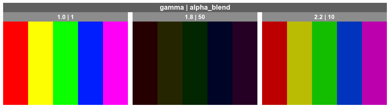
And the plot is executed as follows:
fcp.imshow(df, imgs=imgs, wrap=['gamma', 'alpha_blend'], ncol=3, ws_col=15)
Basic image display#
RGB#
RGB data must be stored in a numpy array. For a single image, it can be passed as the primary arg to the imshow plotting function, along with any other desired kwargs to fine tune the final result:
[ ]:
fcp.imshow(img_rgb, ax_size=[600, 600])
img_rgb.shape

(1000, 2000, 3)
when specifying
ax_sizethe aspect ratio of the original data will be preserved and the larger value between actual height or width will adopt the specified height or widthtick labels are disable by default for
imshow(usetick_labels_major=Trueto enable)
RAW / Grayscale#
fivecentplots can also be used to display 2D RAW/grayscale image data. For this example, we first covert the above RGB image into a scaled 16-bit grayscale pd.DataFrame using an fcp.utilities functions:
img_raw = fcp.utilities.img_grayscale(img_rgb, as_df=True)
img_raw
| 0 | 1 | 2 | 3 | 4 | 5 | 6 | 7 | 8 | 9 | ... | 1990 | 1991 | 1992 | 1993 | 1994 | 1995 | 1996 | 1997 | 1998 | 1999 | |
|---|---|---|---|---|---|---|---|---|---|---|---|---|---|---|---|---|---|---|---|---|---|
| 0 | 56773 | 56773 | 56773 | 56773 | 56773 | 56773 | 56773 | 56773 | 56773 | 56773 | ... | 56516 | 56516 | 56516 | 56516 | 56516 | 56516 | 56516 | 56516 | 56516 | 56516 |
| 1 | 56773 | 56773 | 56773 | 56773 | 56773 | 56773 | 56773 | 56773 | 56516 | 56516 | ... | 56516 | 56516 | 56516 | 56516 | 56516 | 56516 | 56516 | 56516 | 56516 | 56516 |
| 2 | 56773 | 56773 | 56773 | 56773 | 56773 | 56773 | 56773 | 56773 | 56516 | 56516 | ... | 56516 | 56516 | 56516 | 56516 | 56516 | 56516 | 56516 | 56516 | 56516 | 56516 |
| 3 | 56773 | 56773 | 56773 | 56773 | 56773 | 56773 | 56773 | 56773 | 56516 | 56516 | ... | 56516 | 56516 | 56516 | 56516 | 56516 | 56516 | 56516 | 56516 | 56516 | 56516 |
| 4 | 56773 | 56773 | 56773 | 56773 | 56773 | 56773 | 56773 | 56773 | 56773 | 56773 | ... | 56516 | 56516 | 56516 | 56516 | 56516 | 56516 | 56516 | 56516 | 56516 | 56516 |
| ... | ... | ... | ... | ... | ... | ... | ... | ... | ... | ... | ... | ... | ... | ... | ... | ... | ... | ... | ... | ... | ... |
| 995 | 25661 | 24890 | 23862 | 23348 | 23183 | 22670 | 21642 | 20871 | 20555 | 20298 | ... | 54295 | 54295 | 54295 | 54295 | 54295 | 54295 | 54038 | 54038 | 54038 | 54038 |
| 996 | 25404 | 24633 | 23862 | 23348 | 23183 | 22413 | 21642 | 20871 | 20555 | 20298 | ... | 54295 | 54295 | 54295 | 54295 | 54295 | 54295 | 54038 | 54038 | 54038 | 54038 |
| 997 | 25147 | 24633 | 23862 | 23348 | 22926 | 22413 | 21642 | 21128 | 20555 | 20298 | ... | 54295 | 54295 | 54295 | 54295 | 54295 | 54295 | 54038 | 54038 | 54038 | 54038 |
| 998 | 24890 | 24376 | 23862 | 23091 | 22670 | 22156 | 21385 | 21128 | 20298 | 20041 | ... | 54295 | 54295 | 54038 | 54038 | 54038 | 54038 | 54295 | 54295 | 54295 | 54295 |
| 999 | 24633 | 24376 | 23862 | 23091 | 22670 | 22156 | 21385 | 21128 | 20298 | 20041 | ... | 54295 | 54295 | 54038 | 54038 | 54038 | 54038 | 54295 | 54295 | 54295 | 54295 |
1000 rows × 2000 columns
fcp.imshow(img_raw, ax_size=[600, 600], title='Fake RAW, Fake Pirate')

Note
imshow uses the “gray” colormap by default for single-channel RAW images
Colors#
This section applies only to single-channel image data
Color map#
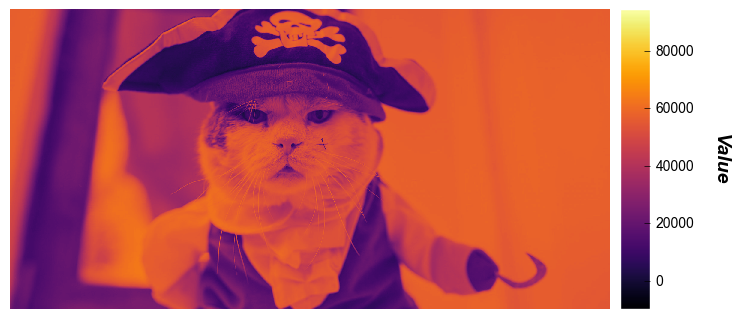
We can add any standard color map from matplotlib to an image using keyword cmap:
fcp.imshow(img_raw, cmap='inferno', ax_size=[600, 600])

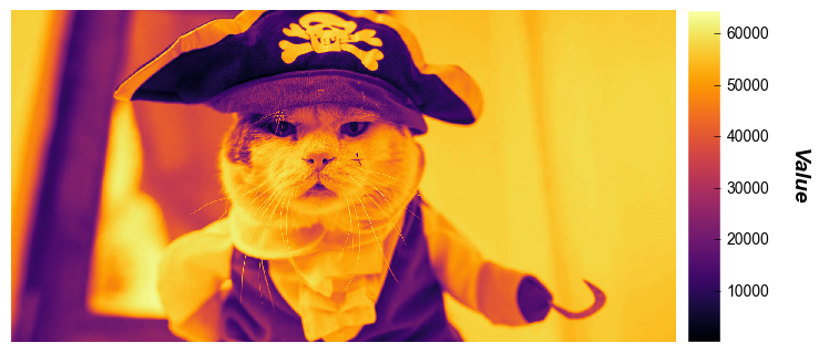
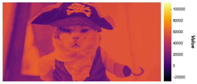
Colorbar#
We can also add a colorbar to the image showing the z-range with the keyword cbar=True
fcp.imshow(img_raw, cmap='inferno', ax_size=[600, 600], cbar=True)
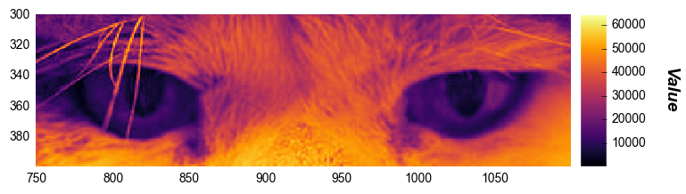
Cropping#
For both single and multi-channel images, we can crop (i.e., zoom in) the image by applying x and y limits. Note that:
xapplies to the image columnsyapplies to the image rowsimage data follows the common convention of starting with “row 0” at the top of the image →
yvalues increase from top to bottom
fcp.imshow(img_raw, cmap='inferno', cbar=True, ax_size=[600, 600], xmin=750, xmax=1100, ymin=300, ymax=400, tick_labels_major=True)
Caution
Private eyes
They’re watching you
They see your every move
Zooming can be achieved by changing the ax_size values for the cropped image. We can also add axes labels:
fcp.imshow(img_rgb, ax_size=[1000, 600], xmin=1400, xmax=1850, ymin=750, ymax=2E20, tick_labels_major=True, label_x='Cat hook pixels', label_y='Image Rows')
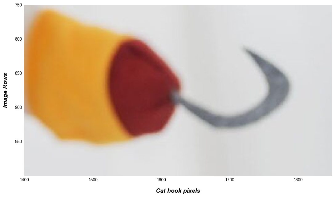
Note
If a crop limit exceeds the actual dimensions of the image, the min or max value is automatically used instead
Contrast stretching#
This section applies only to single-channel image data
In some cases (such as RAW image sensor data analysis) it is helpful to adjust the colormap limits in order to “stretch” the contrast. This can be done via the z axis limits. In this example, we stretch +/-3 standard deviations from the mean pixel value.
# First calculate the mean and std to help define stretching limits
uu = img_raw.stack().mean()
ss = img_raw.stack().std()

# Plot with stretching
fcp.imshow(img_raw, cmap='inferno', cbar=True, ax_size=[600, 600], zmin=uu-3*ss, zmax=uu+3*ss)
imshow plots in fivecentplots also provides a convenient kwarg called stretch which calculates a numerical multiplier of the standard deviation above and below the mean to set new z-limits (the same thing that was done manually above). stretch can be a single value of std dev which is interpreted as +/- that value or a 2-value list with the lower and higher std deviation respectively. First, we consider a +/- 4 sigma stretch as above:
fcp.imshow(img_raw, cmap='inferno', cbar=True, ax_size=[600, 600], stretch=4)
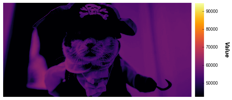
Now we show a single-sided stretch that applies a 3 * std dev increase to the upper z-limit:
fcp.imshow(img_raw, cmap='inferno', cbar=True, ax_size=[600, 600], stretch=[0, 3])
Width/Height Ratio#
By default, fivecentplots will preserve the width to height ratio of the original image. However, this can be overriden if desired via the keyword wh_ratio:
fcp.imshow(img_raw, wh_ratio=1)

Split color planes#
This section applies only to single-channel image data
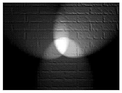
When analyzing Bayer-type images, it is often useful to split the image data based on the color-filter array pattern used on the image sensor. fivecentplots provides a simple utility function to do this and imshow can be used to display the result. Consider the following image:

First we read the image from the world-wide web and convert into a Bayer-like RAW image (rough hack for the purposes of this example):
[ ]:
url = 'https://upload.wikimedia.org/wikipedia/commons/2/28/RGB_illumination.jpg'
img_rgb_sp = imageio.imread(url)
img_raw_sp = fcp.utilities.rgb2bayer(img_rgb_sp)
fcp.imshow(img_raw_sp)
img_raw_sp
array([[ 0,  0,  0, ..., 34,  1,  1],
       [ 0, 32,  0, ...,  2, 67,  0],
       [ 0,  0,  0, ..., 36,  1,  0],
       ...,
       [ 0,  0,  0, ...,  0,  7,  0],
       [ 0,  0,  0, ...,  0,  7,  0],
       [ 0,  0,  0, ...,  0,  7,  0]], dtype=uint8)
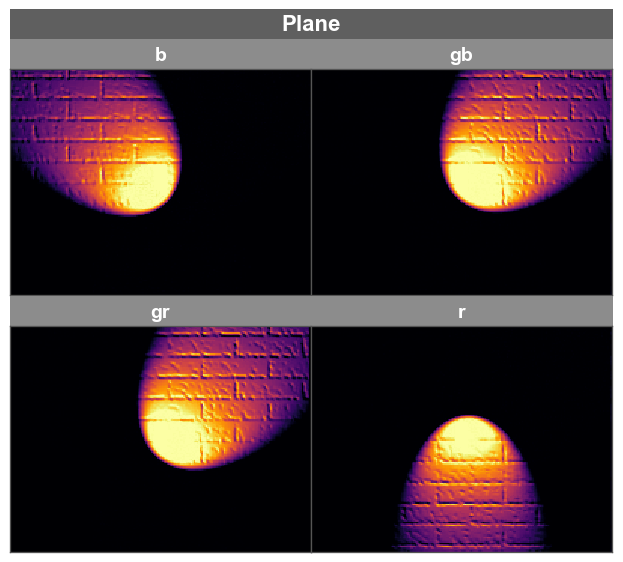
fcp.imshow has a built-in hook to separate RAW single-channel data into discrete color planes if the CFA pattern of the RAW data is supplied with the keyword cfa. This automatically creates a new grouping column for the data called “Plane”, which was can use to separate the color planes into discrete subplots for visualization.
Note
Only CFAs with a 2x2 grid of colors is supported
fcp.imshow(img_raw_sp, cmap='inferno', ax_size=[300, 300], cfa='rggb', wrap='Plane', ax_edge_width=1, ax_edge_color='#555555')
Grouped Images#
As explained in Section 2, to enable the powerful grouping / filtering / automatic-color-plane-splitting functionality of fivecentplots for sets of multiple images in an efficient manner, we cannot rely only on pd.DataFrames. Instead, we use simple pd.DataFrames for unique grouping information only and use a dictionary of np.arrays to store the actual image data.
Simple grouping example#
Let’s create a simple side-by-side of our beloved pirate cat with the same image’s inverse. First, we create a pd.DataFrame with a basic text label to distinguish the two “cases” and a numeric index:
df = pd.DataFrame({'case': ['this is Gary', 'this is inverse Gary']}, index=[0, 1])
df
| case | |
|---|---|
| 0 | this is Gary |
| 1 | this is inverse Gary |
Next, we make a dictionary with two entries: (1) the original image and (2) the inverse image. Remember, that the dictionary keys must match the row indices of our df above:
imgs = {}
imgs[0] = img_rgb
imgs[1] = ((1 - img_rgb / 255) * 255).astype(np.uint16)
imgs
{0: array([[[220, 221, 223],
         [220, 221, 223],
         [220, 221, 223],
         ...,
         [219, 220, 222],
         [219, 220, 222],
         [219, 220, 222]],

        [[220, 221, 223],
         [220, 221, 223],
         [220, 221, 223],
         ...,
         [219, 220, 222],
         [219, 220, 222],
         [219, 220, 222]],

        [[220, 221, 223],
         [220, 221, 223],
         [220, 221, 223],
         ...,
         [219, 220, 222],
         [219, 220, 222],
         [219, 220, 222]],

        ...,

        [[108,  95,  86],
         [106,  93,  84],
         [103,  90,  81],
         ...,
         [209, 211, 210],
         [209, 211, 210],
         [209, 211, 210]],

        [[107,  94,  85],
         [105,  92,  83],
         [103,  90,  81],
         ...,
         [210, 212, 211],
         [210, 212, 211],
         [210, 212, 211]],

        [[106,  93,  84],
         [105,  92,  83],
         [103,  90,  81],
         ...,
         [210, 212, 211],
         [210, 212, 211],
         [210, 212, 211]]], dtype=uint8),
 1: array([[[ 34,  33,  32],
         [ 34,  33,  32],
         [ 34,  33,  32],
         ...,
         [ 36,  34,  32],
         [ 36,  34,  32],
         [ 36,  34,  32]],

        [[ 34,  33,  32],
         [ 34,  33,  32],
         [ 34,  33,  32],
         ...,
         [ 36,  34,  32],
         [ 36,  34,  32],
         [ 36,  34,  32]],

        [[ 34,  33,  32],
         [ 34,  33,  32],
         [ 34,  33,  32],
         ...,
         [ 36,  34,  32],
         [ 36,  34,  32],
         [ 36,  34,  32]],

        ...,

        [[147, 160, 169],
         [148, 162, 171],
         [152, 164, 174],
         ...,
         [ 46,  44,  45],
         [ 46,  44,  45],
         [ 46,  44,  45]],

        [[147, 161, 170],
         [150, 163, 172],
         [152, 164, 174],
         ...,
         [ 45,  42,  44],
         [ 45,  42,  44],
         [ 45,  42,  44]],

        [[148, 162, 171],
         [150, 163, 172],
         [152, 164, 174],
         ...,
         [ 45,  42,  44],
         [ 45,  42,  44],
         [ 45,  42,  44]]], dtype=uint16)}
Now we plot. Pass the grouping label pd.DataFrame as the primary arg to fcp.imshow and the dictionary to the special kwarg called imgs:
fcp.imshow(df, imgs=imgs, wrap='case')

More advanced example#
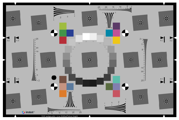
Let’s consider a more complicated example with multiple grouping factors using an ISO 12233 eSFR chart:
base_img = imageio.imread('https://www.imatest.com/wp-content/uploads/2011/11/new_ISO-12233_enh_wedges_3_2_sRGB.png')[12:-12, 15:-15, 0:3]
fcp.imshow(base_img, ax_size=[600, 600])
Now we apply various combinations of Gaussian blur, random noise, and gain to the base image. For each iteration of our processing loop, we need to do two things:
pd.concata new row containing thekernel,sigma, andgainvalues. Initially, we ignore the row index but after the loop we usedf.reset_index()to make a numerical index for each rowtransform the base image and store the result in an
imgsdictionary with a numerical key
which yields a data set of 32 images for plotting with imshow.
Although the specifics of this example are a bit silly, one can readily see the power of fivecentplots for analyzing complex image processing experiments.
df = pd.DataFrame()
imgs = {}
for (kernel, sigma, gain) in itertools.product([1, 3, 5, 7], [0, 0.5, 1, 2], [0.5, 1]):
    df = pd.concat([df, pd.DataFrame({'kernel': kernel, 'sigma': sigma, 'gain': gain}, index=[0])])
    noise = np.random.normal(0, sigma, base_img.shape)
    imgs[len(imgs)] = cv2.GaussianBlur((base_img * gain + noise).astype(np.uint8), (kernel, kernel), 0)
df = df.reset_index()
df
| index | kernel | sigma | gain | |
|---|---|---|---|---|
| 0 | 0 | 1 | 0.0 | 0.5 |
| 1 | 0 | 1 | 0.0 | 1.0 |
| 2 | 0 | 1 | 0.5 | 0.5 |
| 3 | 0 | 1 | 0.5 | 1.0 |
| 4 | 0 | 1 | 1.0 | 0.5 |
| 5 | 0 | 1 | 1.0 | 1.0 |
| 6 | 0 | 1 | 2.0 | 0.5 |
| 7 | 0 | 1 | 2.0 | 1.0 |
| 8 | 0 | 3 | 0.0 | 0.5 |
| 9 | 0 | 3 | 0.0 | 1.0 |
| 10 | 0 | 3 | 0.5 | 0.5 |
| 11 | 0 | 3 | 0.5 | 1.0 |
| 12 | 0 | 3 | 1.0 | 0.5 |
| 13 | 0 | 3 | 1.0 | 1.0 |
| 14 | 0 | 3 | 2.0 | 0.5 |
| 15 | 0 | 3 | 2.0 | 1.0 |
| 16 | 0 | 5 | 0.0 | 0.5 |
| 17 | 0 | 5 | 0.0 | 1.0 |
| 18 | 0 | 5 | 0.5 | 0.5 |
| 19 | 0 | 5 | 0.5 | 1.0 |
| 20 | 0 | 5 | 1.0 | 0.5 |
| 21 | 0 | 5 | 1.0 | 1.0 |
| 22 | 0 | 5 | 2.0 | 0.5 |
| 23 | 0 | 5 | 2.0 | 1.0 |
| 24 | 0 | 7 | 0.0 | 0.5 |
| 25 | 0 | 7 | 0.0 | 1.0 |
| 26 | 0 | 7 | 0.5 | 0.5 |
| 27 | 0 | 7 | 0.5 | 1.0 |
| 28 | 0 | 7 | 1.0 | 0.5 |
| 29 | 0 | 7 | 1.0 | 1.0 |
| 30 | 0 | 7 | 2.0 | 0.5 |
| 31 | 0 | 7 | 2.0 | 1.0 |
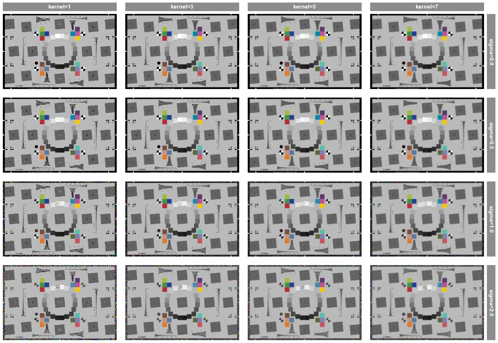
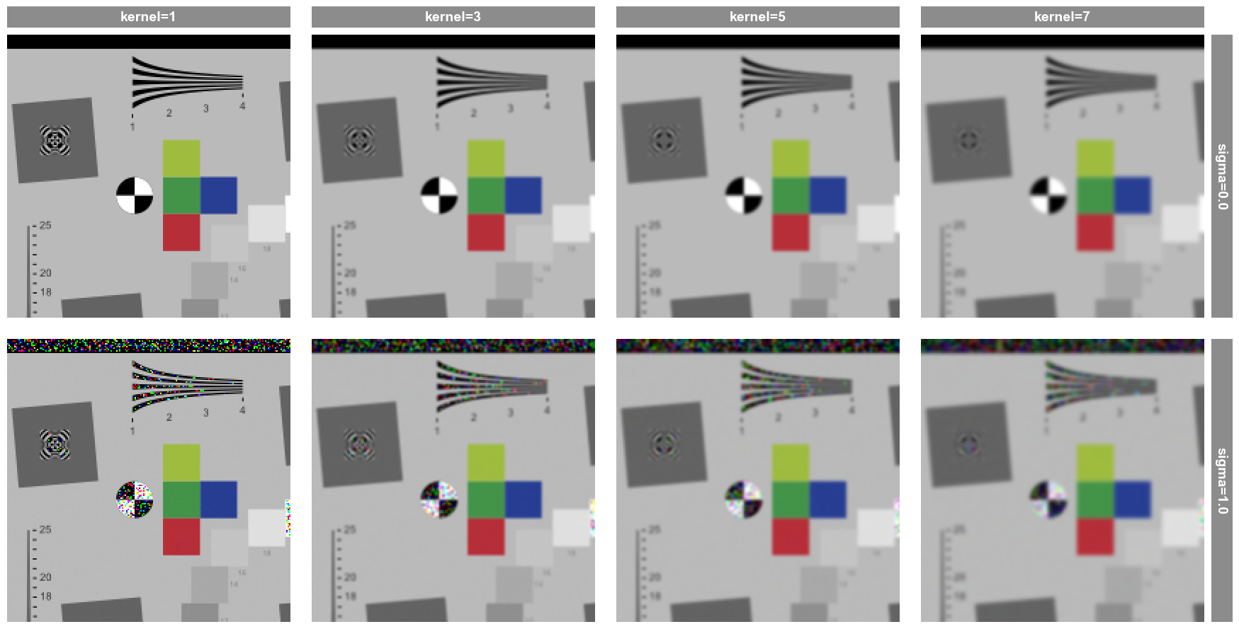
First, we plot all combinations using the kernel value for each column of images, the sigma value for each row of images, and gain as the sole entry in fig_groups which yields a separate plot for each gain value. Notice that the saved filename is printed above each plot, designating the gain value used.
fcp.imshow(df, imgs=imgs, col='kernel', row='sigma', fig_groups='gain', print_filename=True)
Row by sigma by kernel where gain=0.5.png
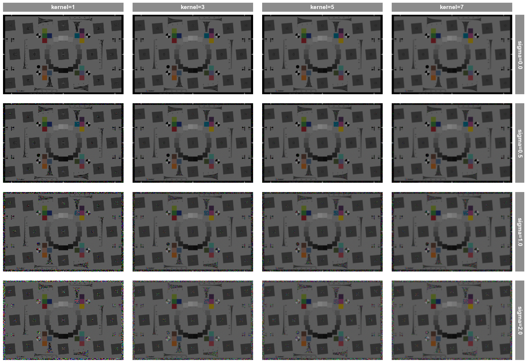
Row by sigma by kernel where gain=1.0.png
Let’s say we are interested in down selecting to only a few cases and zooming in to see the result. This can be accomplished as follows:
fcp.imshow(df, imgs=imgs, col='kernel', row='sigma', filter='gain==1 & kernel < 9 & sigma in [0, 1]', xmin=100, xmax=300, ymax=200)
Note
The above images are zoomed in automatically because our crop dimensions are smaller than the default value for ax_size=[400, 400]
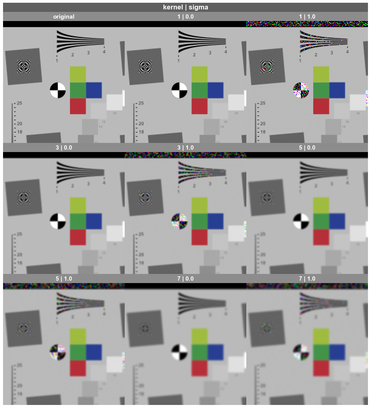
Wrap reference#
Sometimes in image processing analysis, it is helpful to compare results with a reference image. When plotting multiple frame in a wrap plot configuration, reference images can be added as the first or last image in the group by passing a dictionary to the kwarg wrap_reference. This dictionary contains two keys, each with a single value:
Key |
Value |
|---|---|
Reference label name (str) |
|
‘position’ (optional) |
‘first’ (default) or ‘last’ |
fcp.imshow(df, imgs=imgs, wrap=['kernel', 'sigma'], filter='gain==1 & kernel < 9 & sigma in [0, 1]',
           xmin=100, xmax=300, ymax=200,
           wrap_reference={'original': base_img, 'position': 'first'})
Pixel accuracy#
The importance of pixel accuracy when rendering images through fcp.imshow depends on the application. In some cases, we may specifically not want pixel accuracy as it can make the rendered image quality look poor and pixelated. This section describes the options available to address this issue within fivecentplots.
[ ]:
Preserving pixel values#
Let’s create a very basic checkerboard image with only two pixel values, 0 and 255:
n = 40
checkerboard = np.tile(np.array([[0, 255], [255, 0]]), (n//2, n//2))
checkerboard
array([[  0, 255,   0, ..., 255,   0, 255],
       [255,   0, 255, ...,   0, 255,   0],
       [  0, 255,   0, ..., 255,   0, 255],
       ...,
       [255,   0, 255, ...,   0, 255,   0],
       [  0, 255,   0, ..., 255,   0, 255],
       [255,   0, 255, ...,   0, 255,   0]])
fivecentplots will accurately display this pattern if the ax_size keyword matches the array size:
fcp.imshow(checkerboard, ax_size=checkerboard.shape, cmap='inferno')

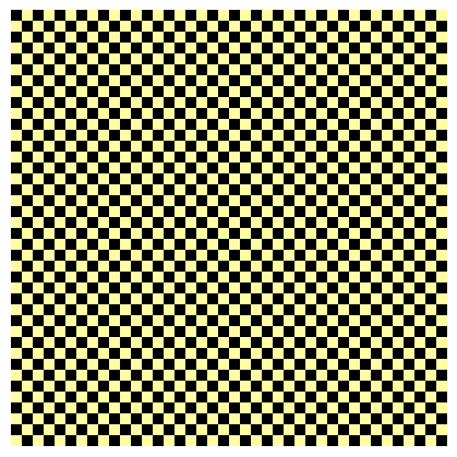
This is hard to visualize, but fortunately, we can size up the image and still preserve the pixel pattern:
fcp.imshow(checkerboard, ax_size=[400, 400], cmap='inferno')
Downsampling#
If the requested ax_size is smaller than the image array size, the plotting backend (in this case matplotlib) performs some downscaling which means the resulting image is no longer pixel accurate:
fcp.imshow(checkerboard, ax_size=[17, 17], cmap='inferno')

The above image is small but careful inspection shows that the black squares are not uniformly sized. We can illustrate this better by saving the images and reading them back, stripping off the plot figure border, and converting to grayscale:
fcp.imshow(checkerboard, ax_size=[40, 40], cmap='inferno', filename='checkerboard_40.png', inline=False, save=True)
fcp.imshow(checkerboard, ax_size=[17, 17], cmap='inferno', filename='checkerboard_17.png', inline=False, save=True)
checkerboard_40 = fcp.utl.img_grayscale(imageio.imread('checkerboard_40.png')[10:-10, 10:-10], bit_depth=8)
checkerboard_17 = fcp.utl.img_grayscale(imageio.imread('checkerboard_17.png')[10:-10, 10:-10], bit_depth=8)
The original image:
checkerboard_40
array([[  0, 243,   0, ..., 243,   0, 243],
       [243,   0, 243, ...,   0, 243,   0],
       [  0, 243,   0, ..., 243,   0, 243],
       ...,
       [243,   0, 243, ...,   0, 243,   0],
       [  0, 243,   0, ..., 243,   0, 243],
       [243,   0, 243, ...,   0, 243,   0]], dtype=uint16)
And the shrunk image:
checkerboard_17
array([[  0,   0,   0, 243, 243, 243,   0,   0, 243, 243, 243,   0,   0,
          0, 243, 243, 243],
       [  0,   0,   0, 243, 243, 243,   0,   0, 243, 243, 243,   0,   0,
          0, 243, 243, 243],
       [  0,   0,   0, 243, 243, 243,   0,   0, 243, 243, 243,   0,   0,
          0, 243, 243, 243],
       [243, 243, 243,   0,   0,   0, 243, 243,   0,   0,   0, 243, 243,
        243,   0,   0,   0],
       [243, 243, 243,   0,   0,   0, 243, 243,   0,   0,   0, 243, 243,
        243,   0,   0,   0],
       [243, 243, 243,   0,   0,   0, 243, 243,   0,   0,   0, 243, 243,
        243,   0,   0,   0],
       [  0,   0,   0, 243, 243, 243,   0,   0, 243, 243, 243,   0,   0,
          0, 243, 243, 243],
       [  0,   0,   0, 243, 243, 243,   0,   0, 243, 243, 243,   0,   0,
          0, 243, 243, 243],
       [243, 243, 243,   0,   0,   0, 243, 243,   0,   0,   0, 243, 243,
        243,   0,   0,   0],
       [243, 243, 243,   0,   0,   0, 243, 243,   0,   0,   0, 243, 243,
        243,   0,   0,   0],
       [243, 243, 243,   0,   0,   0, 243, 243,   0,   0,   0, 243, 243,
        243,   0,   0,   0],
       [  0,   0,   0, 243, 243, 243,   0,   0, 243, 243, 243,   0,   0,
          0, 243, 243, 243],
       [  0,   0,   0, 243, 243, 243,   0,   0, 243, 243, 243,   0,   0,
          0, 243, 243, 243],
       [  0,   0,   0, 243, 243, 243,   0,   0, 243, 243, 243,   0,   0,
          0, 243, 243, 243],
       [243, 243, 243,   0,   0,   0, 243, 243,   0,   0,   0, 243, 243,
        243,   0,   0,   0],
       [243, 243, 243,   0,   0,   0, 243, 243,   0,   0,   0, 243, 243,
        243,   0,   0,   0],
       [243, 243, 243,   0,   0,   0, 243, 243,   0,   0,   0, 243, 243,
        243,   0,   0,   0]], dtype=uint16)
Interpolation#
With the matplotlib engine, fivecentplots supports any of the available interpolation schemes via the keyword interp. Here is our checkboard with a terrifically named interpolation scheme:
fcp.imshow(checkerboard, ax_size=[400, 400], cmap='inferno', interp='catrom')
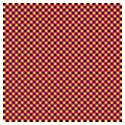
Note
Interpolation can be helpful when plotting high-resolution color images that look pixelated
[ ]: