Styles and formatting
Any Element object in fivecentplots (legend, axis, label, etc.) has certain properties like edge color, fill color, font size that can be styled. Each of the properties can be set by passing the appropriate keyword to the function call to make the plot or by setting a new default value in a custom theme file. Examples of style changes are described below.
Setup
Imports
[1]:
%load_ext autoreload
%autoreload 2
%matplotlib inline
import fivecentplots as fcp
import pandas as pd
import numpy as np
import os, sys, pdb
osjoin = os.path.join
db = pdb.set_trace
Sample data
[2]:
df = pd.read_csv(osjoin(os.path.dirname(fcp.__file__), 'tests', 'fake_data.csv'))
df.head()
[2]:
| Substrate | Target Wavelength | Boost Level | Temperature [C] | Die | Voltage | I Set | I [A] | |
|---|---|---|---|---|---|---|---|---|
| 0 | Si | 450 | 0.2 | 25 | (1,1) | 0.0 | 0.0 | 0.0 |
| 1 | Si | 450 | 0.2 | 25 | (1,1) | 0.1 | 0.0 | 0.0 |
| 2 | Si | 450 | 0.2 | 25 | (1,1) | 0.2 | 0.0 | 0.0 |
| 3 | Si | 450 | 0.2 | 25 | (1,1) | 0.3 | 0.0 | 0.0 |
| 4 | Si | 450 | 0.2 | 25 | (1,1) | 0.4 | 0.0 | 0.0 |
Other
[4]:
SHOW = False
Colors
Fill colors
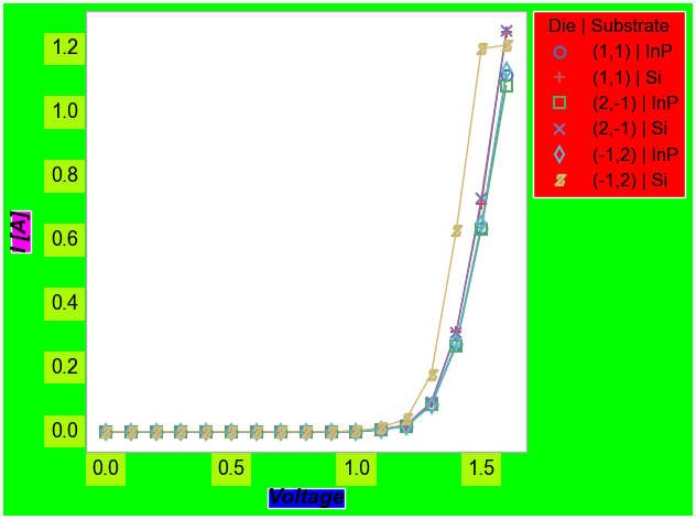
Many elements in a plot are capable of having a fill color (axes, figure background, markers, etc.). These fill colors are accessible using the standard keyword nomenclature of the element name followed by an underscore and the keyword fill_color. All colors are specified using 6-character hex codes.
[5]:
fcp.plot(df=df, x='Voltage', y='I [A]', legend=['Die', 'Substrate'], show=SHOW,
         filter='Target Wavelength==450 & Boost Level==0.2 & Temperature [C]==25',
         fig_fill_color='#00FF00', legend_fill_color='#FF0000', ax_fill_color='#FFFFFF',
         label_x_fill_color='#0000FF', label_y_fill_color='#FF00FF',
         tick_labels_major_fill_color='#AAFB05')
Edge colors
Typical elements
Many elements in a plot also support an edge color (i.e., the border around an object). These edge colors are accessible using the standard keyword nomenclature of the element name followed by _edge_color. Additionally, the width of the edge or border can be specified via keyword using the name of the element followed by _edge_width.
[6]:
fcp.plot(df=df, x='Voltage', y='I [A]', legend=['Die', 'Substrate'], show=SHOW,
         filter='Target Wavelength==450 & Boost Level==0.2 & Temperature [C]==25',
         fig_edge_color='#00FF00', legend_edge_color='#FF0000', ax_edge_color='#FFFFFF',
         label_x_edge_color='#0000FF', label_y_edge_color='#FF00FF',
         tick_labels_major_edge_color='#AAFB05', tick_labels_major_edge_width=5)
Spines
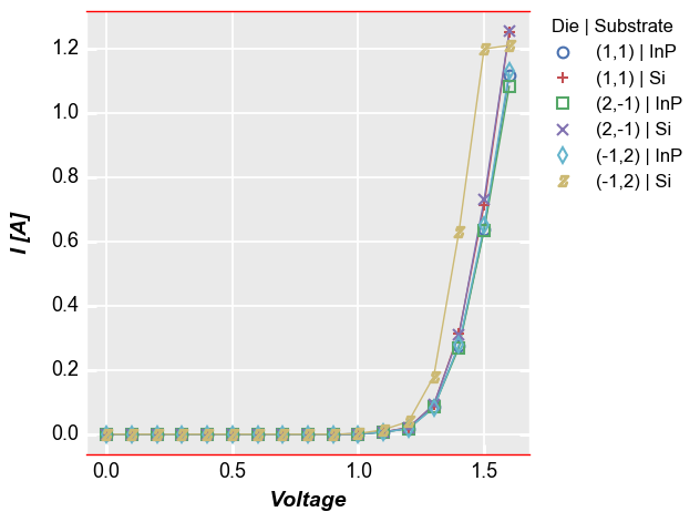
One special case of edge_color is the “spines” or borders around an axis area. In addition to setting the color through the ax_edge_color keyword, individual edges can be turned on or off individually using the keyword spine_<bottom|top|left|right> or spines to simultaneously toggle all of them at once.
[7]:
fcp.plot(df=df, x='Voltage', y='I [A]', legend=['Die', 'Substrate'], show=SHOW,
         filter='Target Wavelength==450 & Boost Level==0.2 & Temperature [C]==25',
         ax_edge_color='#FF0000', spine_left=False, spine_right=False)
Alpha
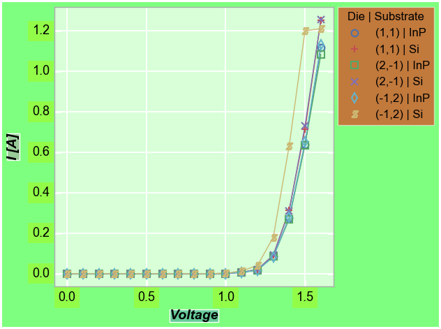
Elements also support alpha for transparency. By default alpha=1 for all elements, but can be changed using the standard keyword nomenclature of the element name followed by an underscore and the keyword fill_alpha or edge_alpha.
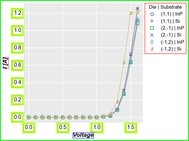
In addition to the fill and edge colors, we can also specify the alpha or opacity of the color. This is done by replacing _fill_color or _edge_color in a given keyword with _fill_alpha or _edge_alpha, respectively. The alpha value is a float ranging from 0 (full opacity) to 1 (no opacity). Internally, the alpha level is converted into hex and appended to the fill or edge color value to make an 8-character hex color code.
Consider the fill example above, with alpha applied to the fill colors:
[8]:
fcp.plot(df=df, x='Voltage', y='I [A]', legend=['Die', 'Substrate'], show=SHOW,
         filter='Target Wavelength==450 & Boost Level==0.2 & Temperature [C]==25',
         fig_fill_color='#00FF00', fig_fill_alpha=0.5,
         legend_fill_color='#FF0000', legend_fill_alpha=0.52,
         ax_fill_color='#FFFFFF', ax_fill_alpha=0.7,
         label_x_fill_color='#0000FF', label_x_fill_alpha=0.2,
         label_y_fill_color='#FF00FF', label_y_fill_alpha=0.2,
         tick_labels_major_fill_color='#AAFB05', tick_labels_major_fill_alpha=0.45)
When adding alpha to plot markers, the legend markers will retain full opacity by default:
[9]:
fcp.plot(df=df, x='Voltage', y='I [A]', legend=['Die', 'Substrate'], show=SHOW,
         filter='Target Wavelength==450 & Boost Level==0.2 & Temperature [C]==25',
         marker_edge_alpha=0.3)
However, there are instances when we want alpha on the plot markers and on the legend markers. To achieve this, use the keyword legend_marker_alpha to set both the edge and fill alpha of the legend markers to a different value:
[10]:
fcp.plot(df=df, x='Voltage', y='I [A]', legend=['Die', 'Substrate'], show=SHOW,
         filter='Target Wavelength==450 & Boost Level==0.2 & Temperature [C]==25',
         marker_edge_alpha=0.3, legend_marker_alpha=0.3)
Line colors
Built-in color list
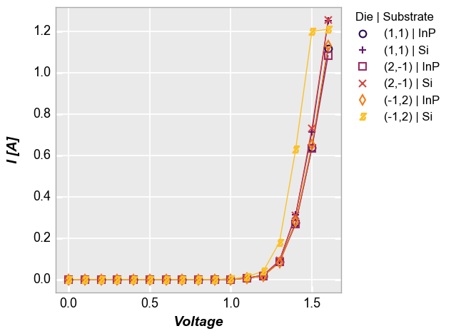
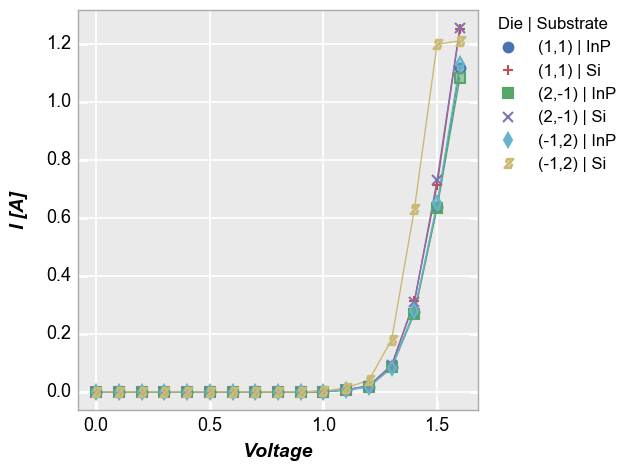
All connecting lines drawn through markers in a plot can be colored. fivecentplots comes with a built-in list of line (and marker) colors (an expanded set of colors from the terrific default palette in the seaborn plotting library). This color pattern repeats indefinetly in case the number of plotted lines exceeds the length of the built-in list.

[11]:
fcp.plot(df=df, x='Voltage', y='I [A]', legend=['Die', 'Substrate'], show=SHOW,
         filter='Target Wavelength==450 & Boost Level==0.2 & Temperature [C]==25')

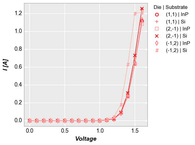
Custom color list
The built-in list of colors can be overriden by passing a list of hex-based color codes to the colors keyword. Like the built-in list, the custom list will also cycle back to the start if there are more lines than colors.
[12]:
fcp.plot(df=df, x='Voltage', y='I [A]', legend=['Die', 'Substrate'], show=SHOW,
         filter='Target Wavelength==450 & Boost Level==0.2 & Temperature [C]==25',
         colors=['#FF0000', '#FF7777', '#FFAAAA'])
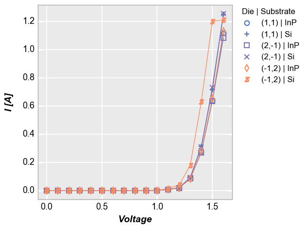
We can also select certain colors from the default color list by index rather than specifying the full hex color code:
[13]:
fcp.plot(df=df, x='Voltage', y='I [A]', legend=['Die', 'Substrate'], show=SHOW,
         filter='Target Wavelength==450 & Boost Level==0.2 & Temperature [C]==25',
         colors=[0, 0, 3, 3, 6, 6])
Colormap
The color list can also be replaced by a discretized colormap using the keyword cmap
[14]:
fcp.plot(df=df, x='Voltage', y='I [A]', legend=['Die', 'Substrate'], show=SHOW,
         filter='Target Wavelength==450 & Boost Level==0.2 & Temperature [C]==25',
         cmap='inferno')
Line styling
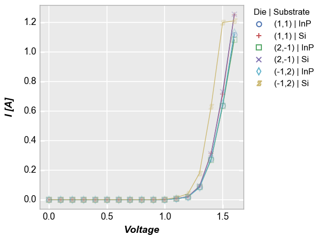
Plot lines do not have a fill or edge so the typical styling parameters like <element name>_fill_color do not exist. Instead, lines have just a unary styling keywords: lines_color, lines_width, lines_style and lines_alpha. In this case, we apply global style settings to all lines in the data set.
[15]:
fcp.plot(df=df, x='Voltage', y='I [A]', legend=['Die', 'Substrate'], show=SHOW,
         filter='Target Wavelength==450 & Boost Level==0.2 & Temperature [C]==25',
         lines_alpha=0.33, lines_style='--', lines_width=3)

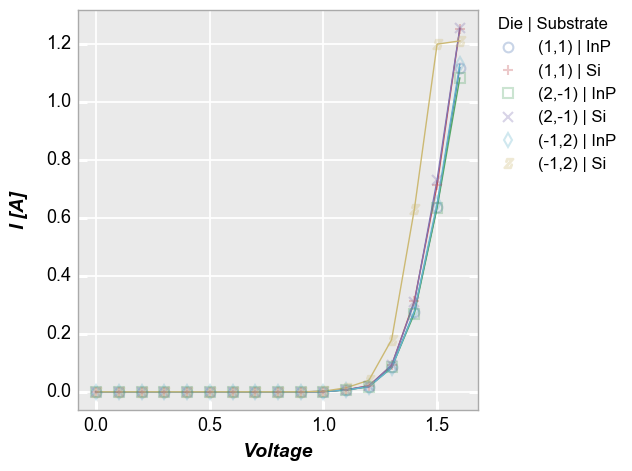
The nomenclature above of lines_<some property> stems from the fact that plot line properties are contained in the lines Element class. However, because this naming scheme may be cumbersome to some users, the non-plural version of these keywords is also supported: * lines_color –> line_color * lines_width –> line_width * lines_style –> line_style * lines_alpha –> line_alpha
[16]:
fcp.plot(df=df, x='Voltage', y='I [A]', legend=['Die', 'Substrate'], show=SHOW,
         filter='Target Wavelength==450 & Boost Level==0.2 & Temperature [C]==25',
         line_alpha=0.33, line_style='--', line_width=3)

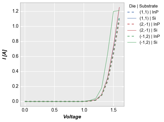
We can also set line styles for each line, instead of applying them globally:
[17]:
fcp.plot(df=df, x='Voltage', y='I [A]', legend=['Die', 'Substrate'], markers=False, show=SHOW,
         filter='Target Wavelength==450 & Boost Level==0.2 & Temperature [C]==25',
         colors=[0, 0, 1, 1, 2, 2],
         lines_width=[3, 1, 3, 1, 3, 1], lines_style=['--', '-'], lines_alpha=[0.6, 1])
Marker colors
A data point marker has both an edge and a fill color, each with its own unique value of transparency (or alpha). By default, marker fill is disabled and marker edge color is matched to the line color with no transparency. However, we can override any of these as shown below.
Change the marker edge color for all markers:
[18]:
fcp.plot(df=df, x='Voltage', y='I [A]', legend=['Die', 'Substrate'], show=SHOW,
         filter='Target Wavelength==450 & Boost Level==0.2 & Temperature [C]==25',
         marker_edge_color=['#555555'])
All a custom fill color:
[19]:
fcp.plot(df=df, x='Voltage', y='I [A]', legend=['Die', 'Substrate'], show=SHOW,
         filter='Target Wavelength==450 & Boost Level==0.2 & Temperature [C]==25',
         marker_edge_color=['#555555'], marker_fill_color='#FFFFFF')
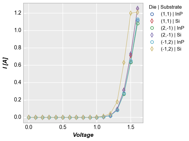
Use the default color scheme with marker fill:
[20]:
fcp.plot(df=df, x='Voltage', y='I [A]', legend=['Die', 'Substrate'], show=SHOW,
         filter='Target Wavelength==450 & Boost Level==0.2 & Temperature [C]==25',
         marker_fill=True)

Add fill alpha:
[21]:
fcp.plot(df=df, x='Voltage', y='I [A]', legend=['Die', 'Substrate'], show=SHOW,
         filter='Target Wavelength==450 & Boost Level==0.2 & Temperature [C]==25',
         marker_fill=True, marker_fill_alpha=0.5)
Boxplot example
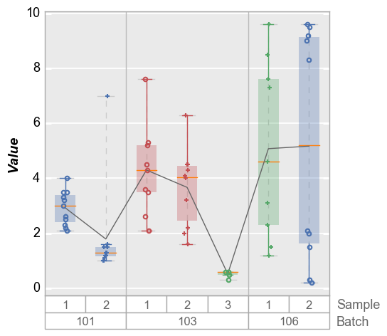
Boxplots have color options for the boxes or violins that are drawn behind the markers:
[22]:
df_box = pd.read_csv(osjoin(os.path.dirname(fcp.__file__), 'tests', 'fake_data_box.csv'))
fcp.boxplot(df=df_box, y='Value', groups=['Batch', 'Sample'], show=SHOW,
            box_fill_color=[0, 0, 1, 1, 2, 2], box_fill_alpha=0.3, box_edge_width=0,
            marker_edge_color=[0, 0, 1, 1, 2, 2], marker_type=['o', '+'],
            box_whisker_color=[0, 0, 1, 1, 2, 2], box_whisker_width=1)
Histogram example
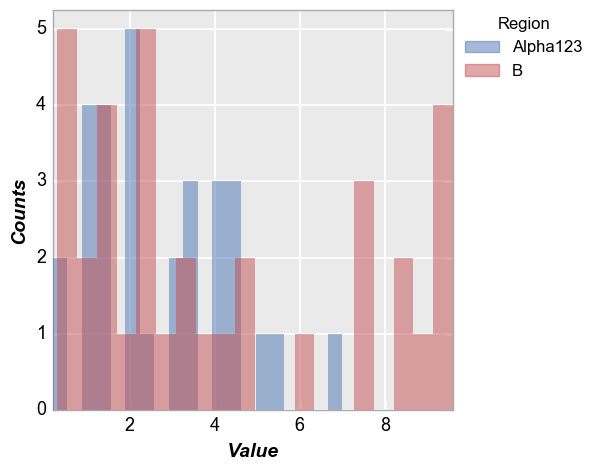
By default, histograms have a fill alpha value of 0.5 (unless overriden by the theme file or keyword). This can easily be tailored for a different style. Compare the default plot:
[23]:
df_hist = pd.read_csv(osjoin(os.path.dirname(fcp.__file__), 'tests', 'fake_data_box.csv'))
fcp.hist(df=df_hist, x='Value', show=SHOW, legend='Region')
with this one, that employs the hist_fill_alpha keyword:
[24]:
fcp.hist(df=df_hist, x='Value', show=SHOW, legend='Region', hist_fill_alpha=1, colors=['#FF0000', '#00FF11'])
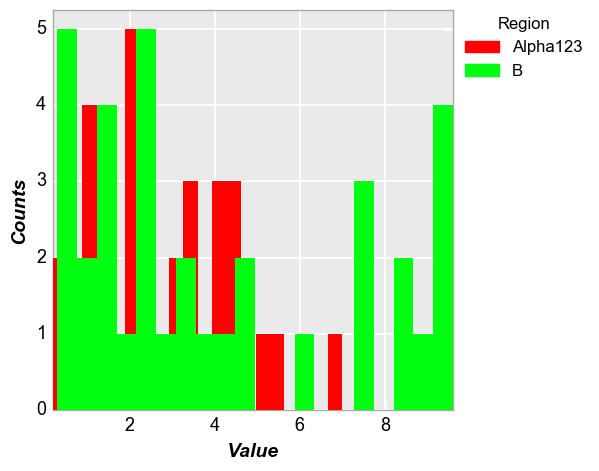
The benefit of transparency is clear in order to visualize both distributions simultaneously.
Markers
Marker type
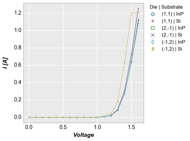
fivecentplots comes with a built-in list of marker styles:

You can specify your own markers by passing a list of marker string names to the markers keyword. These string names can be special characters for the selected plotting engine (for example, with matplotlib as an engine 'd' = diamond) or other alpha-numeric values. As with colors, the marker list will loop back on itself if the number of curves exceeds the number of items in the list.
[25]:
fcp.plot(df=df, x='Voltage', y='I [A]', legend=['Die', 'Substrate'], show=SHOW,
         filter='Target Wavelength==450 & Boost Level==0.2 & Temperature [C]==25',
         markers=['o', 'd'])
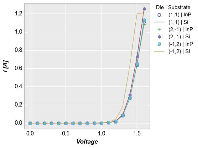
We can also remove markers for specific curves in the legend using the keyword None:
[26]:
fcp.plot(df=df, x='Voltage', y='I [A]', legend=['Die', 'Substrate'], show=SHOW,
         filter='Target Wavelength==450 & Boost Level==0.2 & Temperature [C]==25',
         markers=['o', None, '+', '*', 'B', None])
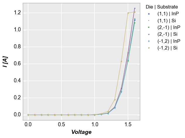
Marker size
The size of the markers within the plot window are controlled by the marker_size keyword. All data sets share the same marker size. Notice that the legend markers do not scale their size with the markers on the plot.
[27]:
fcp.plot(df=df, x='Voltage', y='I [A]', legend=['Die', 'Substrate'], show=SHOW,
         filter='Target Wavelength==450 & Boost Level==0.2 & Temperature [C]==25',
         marker_size=2)
The legend marker size can be controlled independently if needed using the keyword legend_marker_size:
[28]:
fcp.plot(df=df, x='Voltage', y='I [A]', legend=['Die', 'Substrate'], show=SHOW,
         filter='Target Wavelength==450 & Boost Level==0.2 & Temperature [C]==25',
         marker_size=2, legend_marker_size=2)
Fonts
All text elements (plot title, labels, etc.) can be styled via the font attributes associated with the object (see Default Attributes). Please note that the font family “fantasy” below looks an awful lot like comic sans which really should be banned globally.
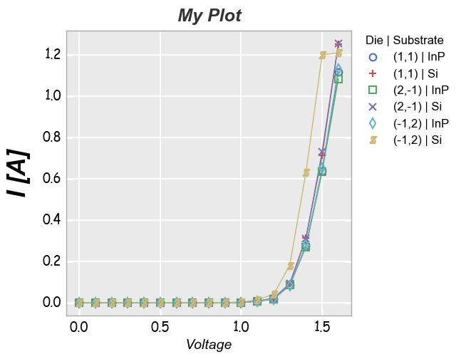
[29]:
fcp.plot(df=df, x='Voltage', y='I [A]', legend=['Die', 'Substrate'], show=SHOW,
         filter='Target Wavelength==450 & Boost Level==0.2 & Temperature [C]==25',
         title='My Plot', title_font_style='italic',
         label_y_font_size=25, label_y_style='normal',
         label_x_font_weight='normal',
         tick_labels_major_font='fantasy')
Themes
Theme files are used to apply user style preferences to all plots without explicitly stating them in keyword arguments. These .py files are populated with dictionaries and lists of style settings. A theme file can be applied globally using the command fcp.set_theme(). Once a theme file is selected, a local copy is made in a /.fivecentplots directory. fivecentplots provides both a “gray” and and “white” theme to get started. You can modify this local file as you wish to get the exact,
consistent look you desire.
The theme file consists of three main parts:
fcp_params: this is a python dictionary that contains anyfcpkeyword argument for which you want to override the default:
fcp_params = {'ax_edge_color': '#aaaaaa',
              'ax_fill_color': '#eaeaea',
              'ax_size': [400,400],  # [width, height]
             }
colors: a list of default colors
colors = ['#000000', '#111111', '#222222']
markers: a list of default markers
markers = ['+', 'o', 'd', '$']
The order of preference for assigning element attributes when plot elements are created is:
keywords in the function call
keywords defined in the local theme file
built-in default values
when using the matplotlib engine, any rcParam overrides you want to apply
Themes are stored in a local user directory (in Windows, this means C:\Users\you\.fivecentplots). The current theme is copied to a new file called defaults.py. All defaults are pulled from this file.
You can switch between themes using the prompt displayed after executing the fcp.set_theme() command. This will open a list of all built-in themes and any custom themes found in your user directory (these files must have a different name than defaults.py). The old theme file will be backed up to defaults_old.py while the new theme file will be copied to defaults.py. You can also pass the name of a theme file directly to set_theme to skip the dialog. However, if you have a
custom theme file in your user directory with the same name as one of the master theme files, set_theme will always give preference to the built-in themes, not your custom theme.
Note: If you create a good theme that you think others can benefit from, feel free to submit it via the github page for this project.
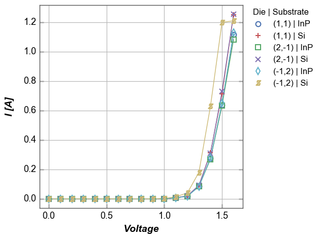
White default theme
[30]:
fcp.set_theme('white')
Previous theme file found! Renaming to "defaults_old.py" and copying new theme...done!
[31]:
fcp.plot(df=df, x='Voltage', y='I [A]', legend=['Die', 'Substrate'], show=SHOW,
         filter='Target Wavelength==450 & Boost Level==0.2 & Temperature [C]==25')

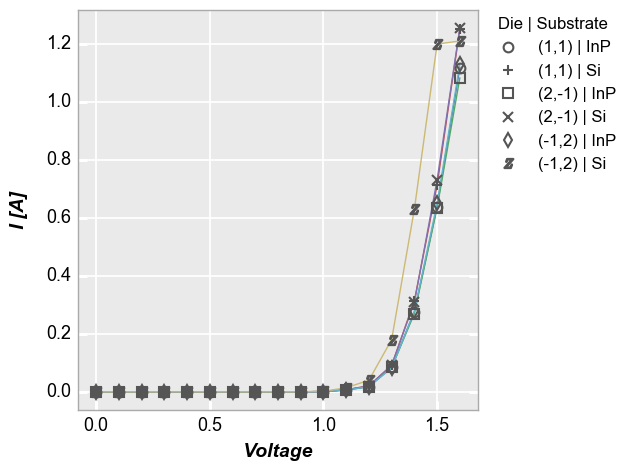
Gray default theme
[32]:
fcp.set_theme('gray')
Previous theme file found! Renaming to "defaults_old.py" and copying new theme...done!
[33]:
fcp.plot(df=df, x='Voltage', y='I [A]', legend=['Die', 'Substrate'], show=SHOW,
         filter='Target Wavelength==450 & Boost Level==0.2 & Temperature [C]==25')

Custom theme files
Currently, fivecentplots only provides a gray (default) and a white theme. However, users can specify there own preferences for the look and feel of a plot by creating a custom theme file. This file has a .py extension and consists of four optional setions:
Figure layout defaults: this is a Python
dictcalledfcp_paramswhich contains the attributes that define the layout (i.e.,ax_edge_colororgrid_major_style)Color scheme: this is an optional Python
listcalledcolorscontaining hex color codes that defines the order of coloring for plots and markers; if blank, the default color scheme is usedMarker scheme: this is an optional Python
listcalledmarkerscontaining symbols to use as markers (the specific symbols should follow the format of the plotting engine being used); if blank, the default color scheme is usedPlotting engine overrides: plotting-engine specific values; for example we might include
rcParamsformatplotlibfonts:
[34]:
import matplotlib as mpl
rcParams = {'font.cursive': ['Apple Chancery',
                             'Textile',
                             'Zapf Chancery',
                             'Sand',
                             'cursive'],
            'font.serif': ['Bitstream Vera Serif',
                           'DejaVu Serif',
                           'New Century Schoolbook',
                           'Century Schoolbook L',
                           'Utopia',
                           'ITC Bookman',
                           'Bookman',
                           'Nimbus Roman No9 L',
                           'Times New Roman',
                           'Times',
                           'Palatino',
                           'Charter',
                           'serif'],
            'agg.path.chunksize': 1000,
            }
mpl.rcParams.update(rcParams)
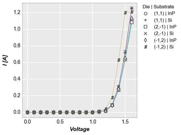
On the fly
As of version 0.4.0, themes can also be swapped on the fly without globally settting the theme using the theme keyword. The value of the keyword is the full path to the alternate theme file or the just the name of a theme file.
In the example below, the default theme is set to gray but we override at the plot call and use the built-in “white” theme:
[35]:
fcp.set_theme('gray')
fcp.plot(df=df, x='Voltage', y='I [A]', legend=['Die', 'Substrate'], show=SHOW,
         filter='Target Wavelength==450 & Boost Level==0.2 & Temperature [C]==25', theme='white')
Previous theme file found! Renaming to "defaults_old.py" and copying new theme...done!
[ ]: