Miscellaneous
Setup
Imports
[1]:
%load_ext autoreload
%autoreload 2
%matplotlib inline
import fivecentplots as fcp
import pandas as pd
import numpy as np
import os, sys, pdb
osjoin = os.path.join
db = pdb.set_trace
Sample data
[2]:
df = pd.read_csv(osjoin(os.path.dirname(fcp.__file__), 'tests', 'fake_data.csv'))
df.head()
[2]:
| Substrate | Target Wavelength | Boost Level | Temperature [C] | Die | Voltage | I Set | I [A] | |
|---|---|---|---|---|---|---|---|---|
| 0 | Si | 450 | 0.2 | 25 | (1,1) | 0.0 | 0.0 | 0.0 |
| 1 | Si | 450 | 0.2 | 25 | (1,1) | 0.1 | 0.0 | 0.0 |
| 2 | Si | 450 | 0.2 | 25 | (1,1) | 0.2 | 0.0 | 0.0 |
| 3 | Si | 450 | 0.2 | 25 | (1,1) | 0.3 | 0.0 | 0.0 |
| 4 | Si | 450 | 0.2 | 25 | (1,1) | 0.4 | 0.0 | 0.0 |
Set theme
(Only needs to be run once)
[3]:
fcp.set_theme('gray')
#fcp.set_theme('white')
Previous theme file found! Renaming to "defaults_old.py" and copying new theme...done!
Other
[4]:
SHOW = False
Text boxes
One or more text boxes can be added to any plot via the text Element class.
Single text box
First we consider a single, non-styled text box:
[5]:
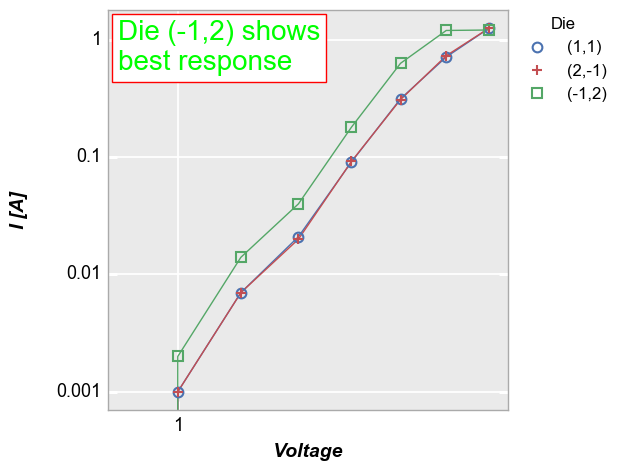
fcp.plot(df, x='Voltage', y='I [A]', ax_scale='loglog', legend='Die', show=SHOW, xmin=0.9,
         filter='Substrate=="Si" & Target Wavelength==450 & Boost Level==0.2 & Temperature [C]==25',
         text='Die (-1,2) shows best response', text_position=[0, 380])

Single text box with styling
We can enhance the look of the text box by accessing color and font properties in the text object using keyword arguments or by definition in a custom theme file. For example, to set the text box fill color, use text_fill_color. The following attributes are defined by default for a text box:
edge_color: nonefill_color: nonefont: sans-seriffont_size: 14font_style: normalfont_weight: normal
[6]:
fcp.plot(df, x='Voltage', y='I [A]', ax_scale='loglog', legend='Die', show=SHOW, xmin=0.9,
         filter='Substrate=="Si" & Target Wavelength==450 & Boost Level==0.2 & Temperature [C]==25',
         text='Die (-1,2) shows\nbest response', text_position=[10, 340], text_font_size=20,
         text_edge_color='#FF0000', text_font_color='#00FF00', text_fill_color='#ffffff')
Multiple text boxes
We can also add multiple text boxes. Because each styling attribute is a RepeatedList, we do not have to explicitly define all attributes for each text box. The provided list of attributes or defaults is cycled through for each text box. Notice below that we define a custom position and font size for each text string, but only one fill_color and only two font_color values. Because these attributes are RepeatedList objects, all elements share the same fill_color and the first
and third text string share the same font_color.
[7]:
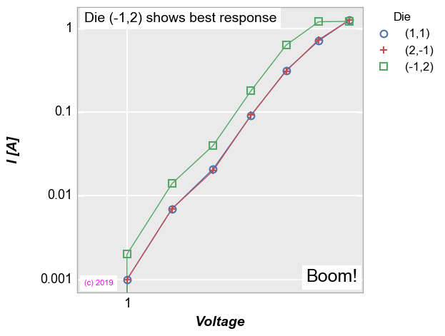
fcp.plot(df, x='Voltage', y='I [A]', ax_scale='loglog', legend='Die', show=SHOW, xmin=0.9,
         filter='Substrate=="Si" & Target Wavelength==450 & Boost Level==0.2 & Temperature [C]==25',
         text=['Die (-1,2) shows best response', '(c) 2019', 'Boom!'],
         text_position=[[10, 379], [10, 10], [320, 15]], text_font_color=['#000000', '#FF00FF'],
         text_font_size=[14, 8, 18], text_fill_color='#FFFFFF')
Position
Coordinate systems
Text box locations can be specified relative to different elements of a given figure:
“axis”: (0,0) is at the lower left corner of the plot window [default]
“figure”: (0,0) is at the lower left corner of the entire figure window
“data”: position is relative to the actual x,y data coordinates
This value is toggled using the text_coordinate keyword. In the examples below, notice how the text_position must change with each coordinate system in order to keep the text box in the same general location.
By “axis” [default]
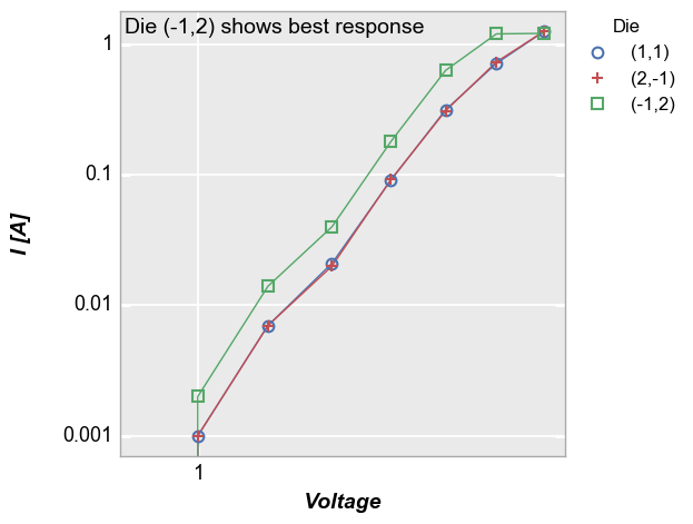
[8]:
fcp.plot(df, x='Voltage', y='I [A]', ax_scale='loglog', legend='Die', show=SHOW, xmin=0.9,
         filter='Substrate=="Si" & Target Wavelength==450 & Boost Level==0.2 & Temperature [C]==25',
         text='Die (-1,2) shows best response', text_position=[0, 380])
By “figure”
[9]:
fcp.plot(df, x='Voltage', y='I [A]', ax_scale='loglog', legend='Die', show=SHOW, xmin=0.9,
         filter='Substrate=="Si" & Target Wavelength==450 & Boost Level==0.2 & Temperature [C]==25',
         text='Die (-1,2) shows best response', text_position=[110, 440], text_coordinate='figure')
By “data”
[10]:
fcp.plot(df, x='Voltage', y='I [A]', ax_scale='loglog', legend='Die', show=SHOW, xmin=0.9,
         filter='Substrate=="Si" & Target Wavelength==450 & Boost Level==0.2 & Temperature [C]==25',
         text='Die (-1,2) shows best response', text_position=[0.903, 1.2], text_coordinate='data')

Units
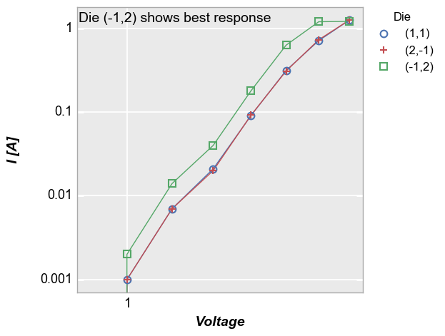
By default, “axis” and “figure” referenced position values are units of pixels. We can cast these into relative units between 0 and 1 (0 and 100%) of scale using the keyword text_units.
[11]:
fcp.plot(df, x='Voltage', y='I [A]', ax_scale='loglog', legend='Die', show=SHOW, xmin=0.9,
         filter='Substrate=="Si" & Target Wavelength==450 & Boost Level==0.2 & Temperature [C]==25',
         text='Die (-1,2) shows best response', text_position=[0, 0.95], text_units='relative')

[ ]: